Hasta ahora, los modelos presentados modelizan el comportamiento de una variable mediante una combinación lineal de parámetros, variables y término error:
\[
Y_t = \beta_0 + \beta_1X_{1,t} + \beta_2X_{2,t} + \ldots + \beta_k X_{k,t} + u_t
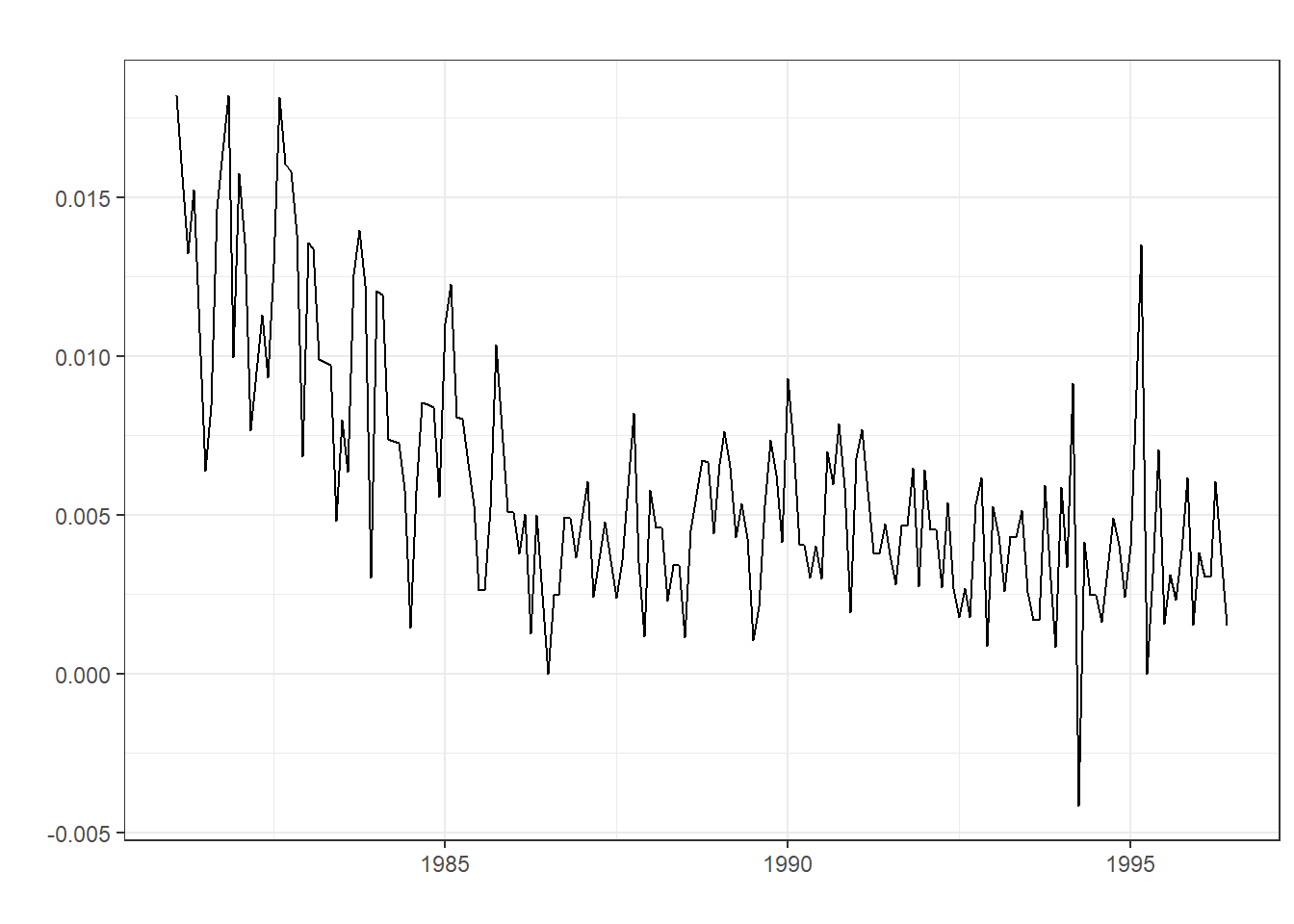
\] Sin embargo, muchas series temporales, como las financieras, presentan un fenómeno conocido como clustering de volatilidad. Esto implica que las series temporales tienen variabilidad cambiante con periodos de alta y baja volatilidad caracterizados por su persistencia.
Esta volatilidad cambiante se puede modelizar a través de la varianza del término error de una serie temporal:
donde ahora la media del término error es constante y cero, pero la varianza es variable y depende de los errores al cuadrado retardados \(p\) periodos (término autorregresivo) y de las perturbaciones aleatorias retardadas \(q\) periodos (término de medias móviles).
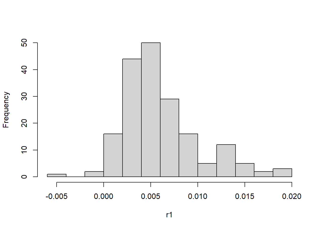
Sin embargo, para que este modelo tenga sentido, lo primero es testar que la serie presente efectos ARCH en sus errores. A menudo, series con distribuciones de probabilidad de colas pesadas y mucha variabilidad suelen presentarlos.
library(forecast, quietly = T)
Warning: package 'forecast' was built under R version 4.2.3
Registered S3 method overwritten by 'quantmod':
  method            from
  as.zoo.data.frame zoo
library(Ecdat, quietly = T)
Warning: package 'Ecdat' was built under R version 4.2.3
Warning: package 'Ecfun' was built under R version 4.2.3
Attaching package: 'Ecfun'
The following object is masked from 'package:forecast':

    BoxCox
The following object is masked from 'package:base':

    sign
Attaching package: 'Ecdat'
The following object is masked from 'package:datasets':

    Orange
library(ggplot2, quietly=T)
Warning: package 'ggplot2' was built under R version 4.2.3
Sin embargo, como siempre un test estadístico formal es necesario para contrastarlo de forma fiable. El test prueba si los parámetros \(\alpha_1, \alpha_2, \ldots, \alpha_j\) de la regresión:
son conjuntamente significativos mediante un estadístico multiplicador de Lagrange (LM), con hipótesis nula \(\alpha_1, \alpha_2, \ldots, \alpha_j = 0\) e hipótesis alternativa de lo contrario.
library(FinTS, quietly = T)
Attaching package: 'zoo'
The following objects are masked from 'package:base':

    as.Date, as.Date.numeric
Attaching package: 'FinTS'
The following object is masked from 'package:forecast':

    Acf
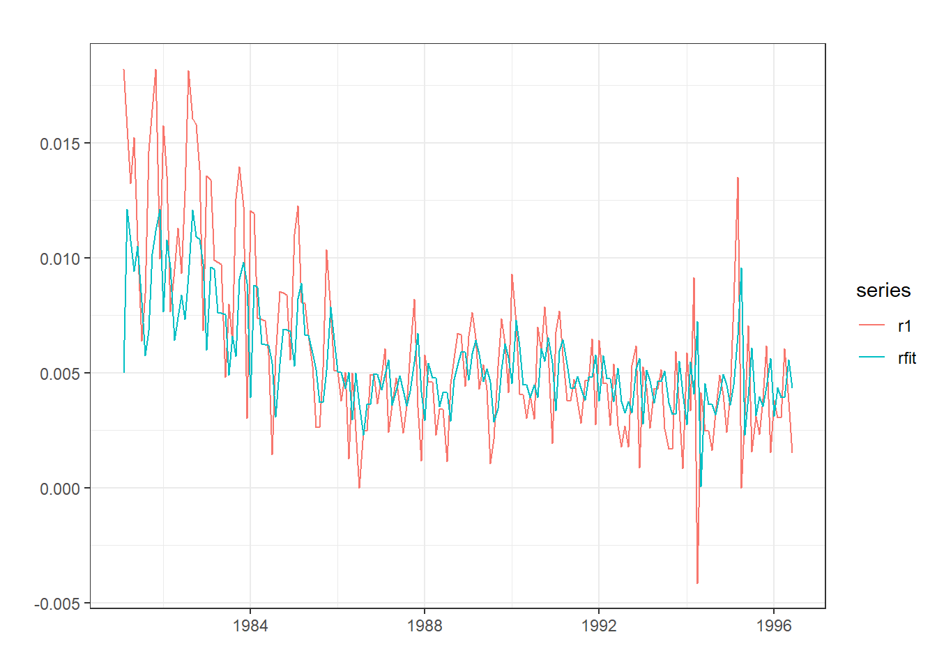
Para modelizar la serie, la elección del orden (\(p\) , \(q\)) de los parámetros se puede hacer por prueba error, analizando cuales de los mismos son estadísticamente significativos. Sin embargo, una opción estandar suele ser el modelo GARCH(1,1).
library(rugarch, quietly = T)
Attaching package: 'rugarch'
The following object is masked from 'package:stats':

    sigma
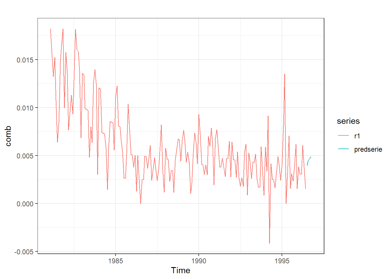
especificacion <-ugarchspec(variance.model=list(model="sGARCH",garchOrder=c(1,1)),mean.model=list(armaOrder=c(1,0)), distribution.model="std") #Modelo GARCH(1,1) y para la serie AR(1).ajuste <-ugarchfit(spec=especificacion, data=r1) #Estimaciónajuste #Resultados del modelo