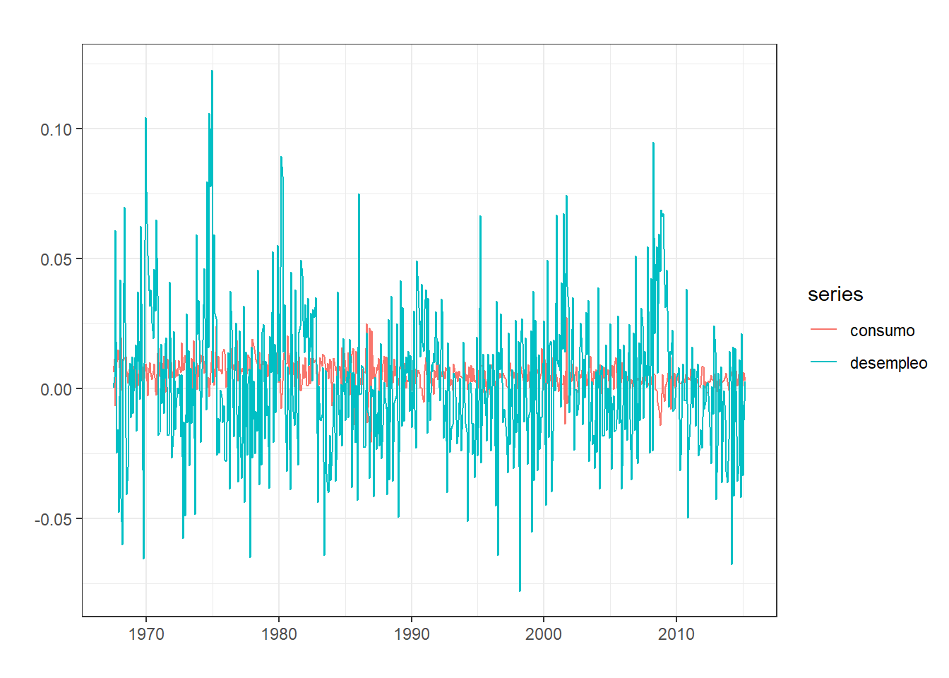
Existen numerosas ocasiones en las cuales las variables guardan relaciones bidireccionales entre sí. Es decir, no solo \(Y\) afecta a \(X\), sino que \(X\) también afecta a \(Y\). Los modelos empleados hasta ahora, no son capaces de capturar dicho comportamiento.
Sin embargo, el modelo de Vectores Autorregresivos o VAR, si que lo permite:
donde se ha escogido un número de variables \(k=2\) y de retardos \(p=1\) por sencillez, pero siendo el modelo generalizable a cualquier conjunto \(k=1,\ldots,K\) de variables aleatorias y \(p=1,\ldots,P\) retardos.
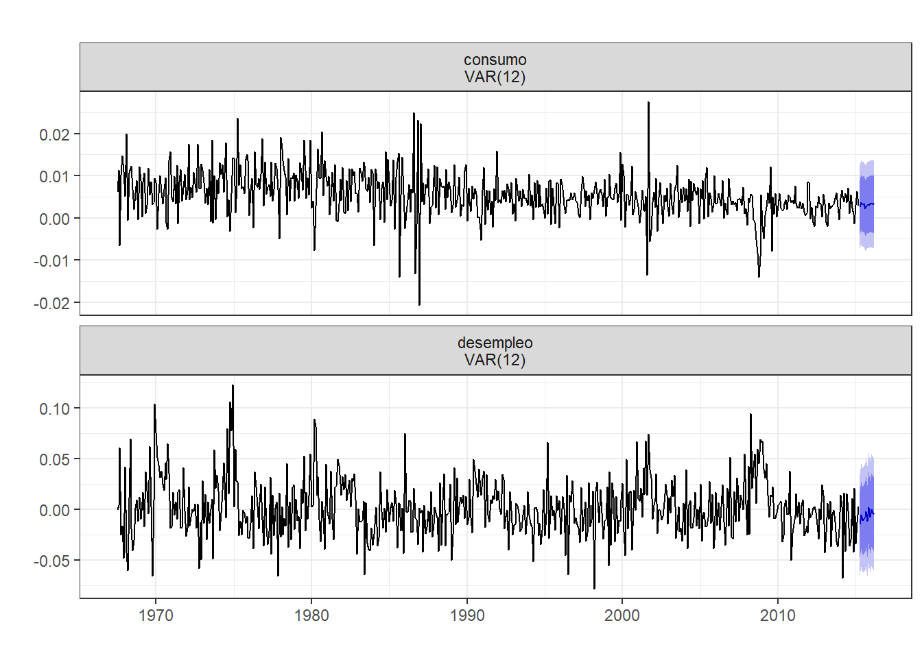
Una vez estimado un modelo VAR, se pueden hacer predicciones. Habitualmente, debido a las relaciones de endogeneidad entre variables que permite, el modelo VAR supera a la mayoría de los modelos en la predicción.
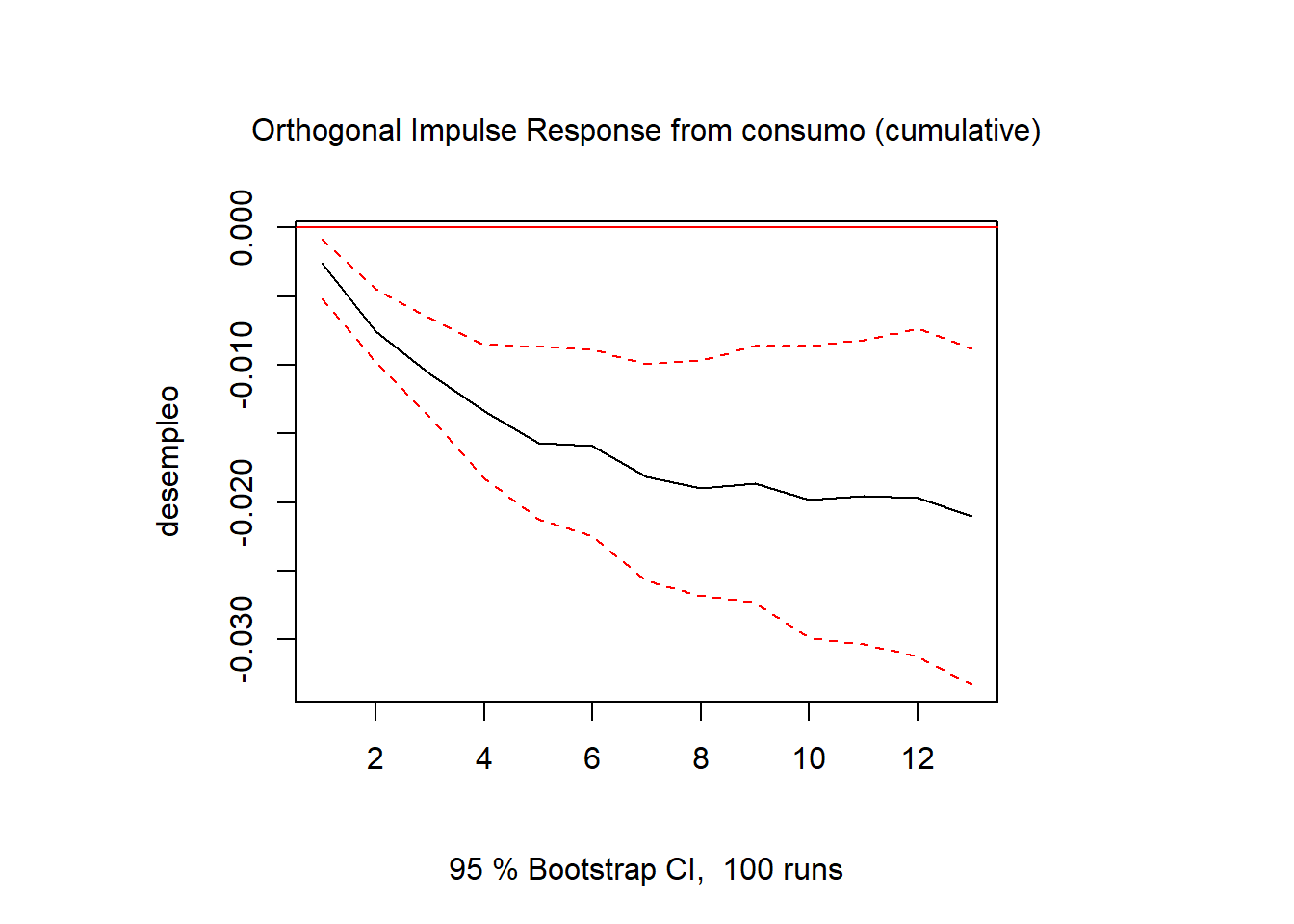
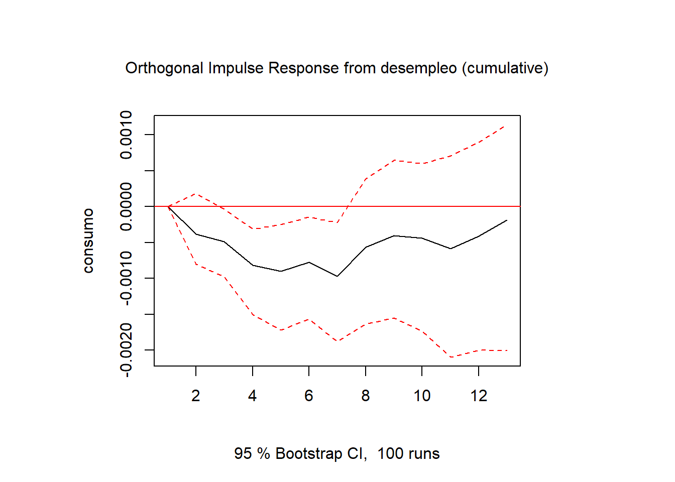
Además, se puede realizar un análisis estructural del modelo. En primer lugar, se pueden obtener las funciones de respuesta al impulso, que miden cuanto responderá una variable ante una innovación de una desviación típica en la otra.
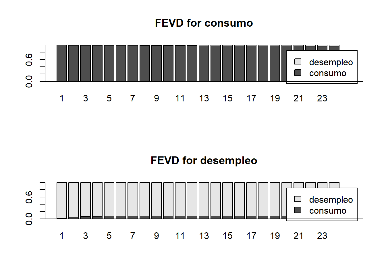
También se puede ejecutar una descomposición de la varianza predicha, con lo que se obtiene una idea de cuanto afecta la varianza del error de una variable en la otra.
Si dos series temporales están cointegradas, en el largo plazo tenderán a coincidir. Sin embargo, en el corto plazo, existirán desviaciones. El modelo de vector de corrección de error VECM, explota este hecho, incluyendo coeficientes a largo plazo, y desviaciones a corto plazo.
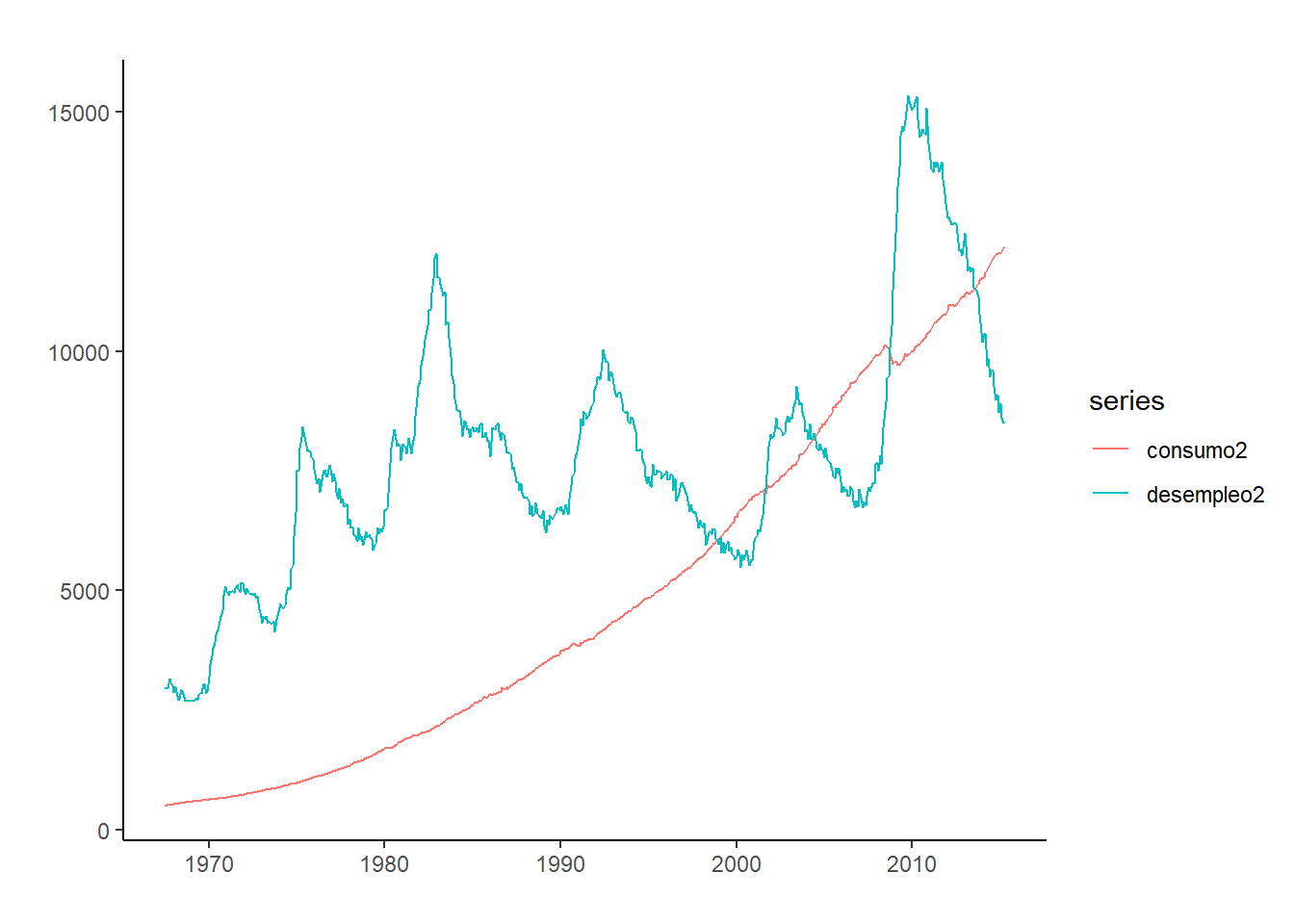
test1 <-ur.df(consumo2) summary(test1)#Serie no es I(0)
###############################################
# Augmented Dickey-Fuller Test Unit Root Test #
###############################################

Test regression none


Call:
lm(formula = z.diff ~ z.lag.1 - 1 + z.diff.lag)

Residuals:
     Min       1Q   Median       3Q      Max
-173.072   -4.184    3.631   13.383  172.732

Coefficients:
            Estimate Std. Error t value Pr(>|t|)
z.lag.1    0.0035417  0.0002348  15.084   <2e-16 ***
z.diff.lag 0.0204848  0.0420327   0.487    0.626
---
Signif. codes:  0 '***' 0.001 '**' 0.01 '*' 0.05 '.' 0.1 ' ' 1

Residual standard error: 25.53 on 570 degrees of freedom
Multiple R-squared:  0.4185,    Adjusted R-squared:  0.4164
F-statistic: 205.1 on 2 and 570 DF,  p-value: < 2.2e-16


Value of test-statistic is: 15.0842

Critical values for test statistics:
      1pct  5pct 10pct
tau1 -2.58 -1.95 -1.62
test2 <-ur.df(diff(consumo2))summary(test2)#Pero si es I(1)
###############################################
# Augmented Dickey-Fuller Test Unit Root Test #
###############################################

Test regression none


Call:
lm(formula = z.diff ~ z.lag.1 - 1 + z.diff.lag)

Residuals:
     Min       1Q   Median       3Q      Max
-122.508   -3.863    5.044   17.788  205.334

Coefficients:
           Estimate Std. Error t value Pr(>|t|)
z.lag.1    -0.33426    0.04099  -8.154 2.26e-15 ***
z.diff.lag -0.40846    0.03847 -10.617  < 2e-16 ***
---
Signif. codes:  0 '***' 0.001 '**' 0.01 '*' 0.05 '.' 0.1 ' ' 1

Residual standard error: 27.61 on 569 degrees of freedom
Multiple R-squared:  0.402, Adjusted R-squared:  0.3999
F-statistic: 191.2 on 2 and 569 DF,  p-value: < 2.2e-16


Value of test-statistic is: -8.1539

Critical values for test statistics:
      1pct  5pct 10pct
tau1 -2.58 -1.95 -1.62
test3 <-ur.df(desempleo2) summary(test3)#Serie no es I(0)
###############################################
# Augmented Dickey-Fuller Test Unit Root Test #
###############################################

Test regression none


Call:
lm(formula = z.diff ~ z.lag.1 - 1 + z.diff.lag)

Residuals:
    Min      1Q  Median      3Q     Max
-840.67 -126.91   -0.81  125.19  789.87

Coefficients:
            Estimate Std. Error t value Pr(>|t|)
z.lag.1    0.0002688  0.0010842   0.248    0.804
z.diff.lag 0.1833904  0.0412105   4.450 1.03e-05 ***
---
Signif. codes:  0 '***' 0.001 '**' 0.01 '*' 0.05 '.' 0.1 ' ' 1

Residual standard error: 212.8 on 570 degrees of freedom
Multiple R-squared:  0.0339,    Adjusted R-squared:  0.03051
F-statistic:    10 on 2 and 570 DF,  p-value: 5.382e-05


Value of test-statistic is: 0.2479

Critical values for test statistics:
      1pct  5pct 10pct
tau1 -2.58 -1.95 -1.62
test4 <-ur.df(diff(desempleo2))summary(test4) #Pero si es I(1)
###############################################
# Augmented Dickey-Fuller Test Unit Root Test #
###############################################

Test regression none


Call:
lm(formula = z.diff ~ z.lag.1 - 1 + z.diff.lag)

Residuals:
    Min      1Q  Median      3Q     Max
-792.17 -118.18   -0.02  123.88  695.86

Coefficients:
           Estimate Std. Error t value Pr(>|t|)
z.lag.1    -0.59759    0.05161 -11.580  < 2e-16 ***
z.diff.lag -0.26782    0.04040  -6.629 7.85e-11 ***
---
Signif. codes:  0 '***' 0.001 '**' 0.01 '*' 0.05 '.' 0.1 ' ' 1

Residual standard error: 205.2 on 569 degrees of freedom
Multiple R-squared:  0.4505,    Adjusted R-squared:  0.4486
F-statistic: 233.3 on 2 and 569 DF,  p-value: < 2.2e-16


Value of test-statistic is: -11.5795

Critical values for test statistics:
      1pct  5pct 10pct
tau1 -2.58 -1.95 -1.62
johansen <-ca.jo(datos2, type="eigen", K=2) #Test de cointegración de johansen.summary(johansen) #Eltest indica al menos una relación de cointegración.
######################
# Johansen-Procedure #
######################

Test type: maximal eigenvalue statistic (lambda max) , with linear trend

Eigenvalues (lambda):
[1] 0.107137493 0.005512336

Values of teststatistic and critical values of test:

          test 10pct  5pct  1pct
r <= 1 |  3.16  6.50  8.18 11.65
r = 0  | 64.82 12.91 14.90 19.19

Eigenvectors, normalised to first column:
(These are the cointegration relations)

              consumo2.l2 desempleo2.l2
consumo2.l2     1.0000000      1.000000
desempleo2.l2  -0.1984701     -2.602472

Weights W:
(This is the loading matrix)

             consumo2.l2 desempleo2.l2
consumo2.d   0.002732568 -6.749625e-05
desempleo2.d 0.002403782  2.819766e-03